Microsoft Excel can be the best tool to work with numbers, data, and information in an organized way if you know the right functions to implement. It has various unique in-built functions and tools to address each data set.

Say, if you want to quickly identify low-stock items in a large inventory spreadsheet, use Excel’s VLOOKUP function to search for specific products and retrieve their quantities.

Or if you have a big list of numbers or words and you need to find something important or make it easier to understand? You can make use of Conditional Formatting.

Let’s Discuss a little on Conditional Formatting

Conditional Formatting helps to make your data stand out, so you can easily see important things or patterns. It’s like having a helper that automatically makes things more noticeable or colorful based on what you tell it to do.

Imagine you have a sheet with random numbers on it. With Conditional Formatting, you can tell Excel, “If a number is bigger than 10, make it turn blue!” Excel will then go through all the numbers and change the ones that are bigger than 10 to blue.

The easiest way to implement Conditional Formatting is with the help of predefined formatting options based on specific criteria. These rules are relatively easier to apply and are suitable for common formatting requirements.

But when you add the concept of formulas in Conditional Formatting, it allows for more customized and flexible formatting options.

But How Exactly Does the Formula Work?

You can leverage Excel’s formula capabilities to define complex conditions based on cell values, other cells, or even external data.

Let’s say you have lists of names and the annual salary for each person. You want to highlight the values on the condition if the salary is greater than or equal to the salary in a specific cell.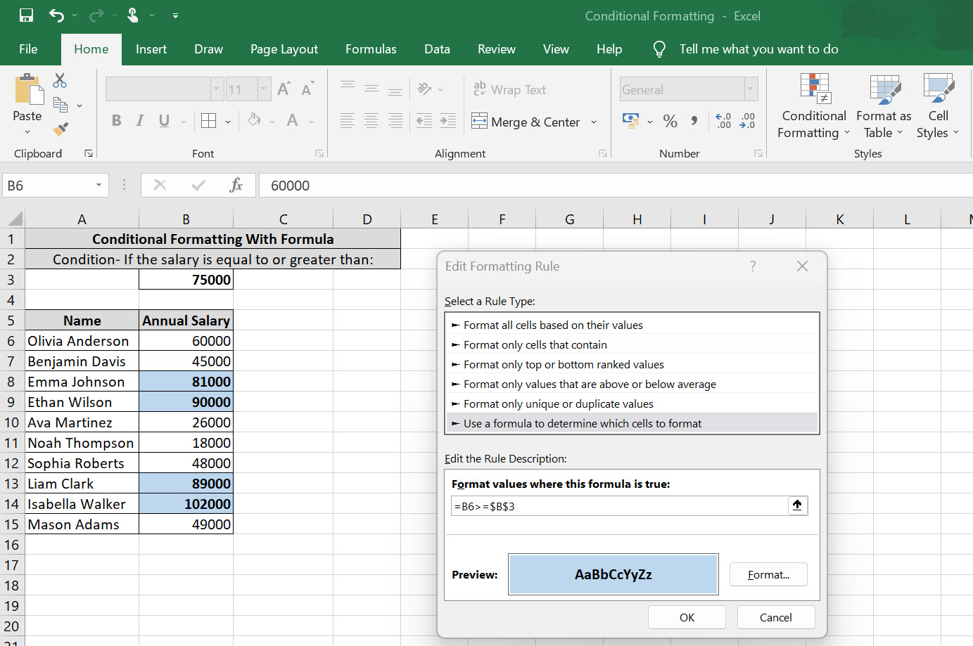

Here is how you can do it:

1. The first thing you need to do is highlight the range you want to format, go to Conditional Formatting and apply a “new rule.”
2. You need to Use a formula to determine which cells to format because the Formatting of Annual Salary Cells is dependent on the value of another cell.
3. Input the formula “=B6>=$B$3″ in the Format values where this formula is true.
4. Under Format, you can select between Number, Font Formatting, Adjust Boarder & Fill Color and click on “OK.“
5. Conditional Formatting is going to check whether the result of the formula is true or false.
6. If it’s true, it’s going to apply to the Formatting that you define (In the above case, the color blue).
7. If it’s false, it’s going to leave the Formatting as is.

Note: The formula that you type is always from the point of view of the first cell in the range that you’ve highlighted. This is from the point of view of B6 in the above case. Excel automatically fixes the sign reference; thus, it is important to double-check the formula before running the function.

Make Your Own Rules

Excel spreadsheet is like a playground, offering endless possibilities to explore and experiment with. As you start fiddling with formulas, you’ll realize that there are multiple ways you can modify data and uncover hidden insights. All you need is basic knowledge, patience, and a curious mind.